Everyone knows MD4 is insecure. Modern attacks can find MD4 collisions almost instantly. It’s easy to forget that the algorithm stood up to a decade and a half of cryptanalysis before Wang et al. broke it open in 2004.

Wang’s attack was the first efficient collision attack on MD4 but not the last; the efficiency of the attack and the clarity of its presentation were both improved by later research. Nevertheless, Wang’s attack has historical significance, and it is included in set 7 of the Cryptopals Challenges.

I’ve been working through Cryptopals lately and I found this to be, without a doubt, the hardest and most engaging challenge in the first 7 sets.

The attack itself is hard to implement; it is also hard to figure out what you’re supposed to implement. That’s why this post is broken up into two parts: this one, which summarizes the attack’s theoretic underpinnings, and a forthcoming second part which details an efficient implementation in Python.

The original paper gives a partial sketch of the attack, plus some example collisions to prove that it works. To work out the details, you have to read between the lines of a challenging paper which (for English speakers) is only available in translation.

Eventually I gave in and started searching for blog posts on the attack; the few I found were not much help. These are written to be the posts I wish I’d found. I had only meant to write one post, but it was getting pretty long so I decided to break it up into two parts: this one, on the theory of the attack, followed by a forthcoming second part detailing an efficient implementation of the attack in Python.

They say you don’t understand something until you can teach it, so these posts are my way of proving to myself that I understand Wang’s attack. I hope someone finds them useful or at least interesting. If they aren’t detailed enough for you, come on out to Seattle and we’ll go through it over beers, coffee, or your beverage of choice.

the basic idea

This attack is a differential attack, meaning we as attackers are trying to find collisions between pairs of messages where the messages also share a fixed difference.

Differential attacks commonly use xor difference, but in this attack we are interested in arithmetic difference; that is to say, we want messages \(m, m'\) such that \(H(m) = H(m')\) and \(m' - m = D\) for some fixed differential \(D\).

This might sound like adding an unnecessary constraint – and it is – but it gives us a powerful way of reframing the problem. This definition makes \(m'\) fully dependent on \(m\) and \(D\), so for the attack to succeed it suffices to identify a set of messages \(S\) such that if \(m \in S\) then \(H(m) = H(m + D)\) with high probability.

Wang’s attack consists of a definition for one such differential \(D\) and a method for arriving at likely elements of the corresponding message set \(S\).

The attack’s supporting theory is centered around an analysis of how certain differentials spread through MD4’s internal state. Supported by a set of simple collisions in the hash function’s round functions, this analysis culminates in a set of (nearly) sufficient conditions for differentials in different parts of the message to “cancel each other out” like waves coming together and destructively interfering.

The result of this analysis is a characterization of the message set \(S\), which is defined by a set of more than one hundred conditions on the hash function’s intermediate states. These together form a set of (almost)¹ sufficient conditions for membership in \(S\). Out of these hundred-odd conditions, the paper prescribes methods for ensuring that a couple of them are met; we are left to figure out the rest on our own.

The result, if we are successful, is that during MD4 computation, differences in the messages’ hashes’ intermediate states will be introduced and erased – that is, the states will be made to diverge and then reconverge – giving rise to collisions.

Before expanding on that idea, let’s review the relevant parts of MD4 itself.

the structure of MD4 (in brief)

MD4 has a 128-bit internal state. Internally, this is represented as four 32-bit state variables. Call them \(a, b, c, d\). These are initialized to certain fixed values. We’ll call those \(a_0, b_0, c_0, d_0\).

MD4 takes 512-bit message blocks. We’re only going to concern ourselves with one-block messages here.²

The message block is broken up into sixteen consecutive 32-bit words, denoted by \(m_0, m_{1}, ..., m_{15}\).

The message block is mixed with the state through a series of three rounds. Each round consists of sixteen steps; each step modifies one of the four state variables as a function of the whole state plus a message word \(m_k\).

Each message word is used exactly once per round. Each of the three rounds uses a different round function. All three round functions have simple algebraic representations.

Here’s what the full process for hashing one block looks like:

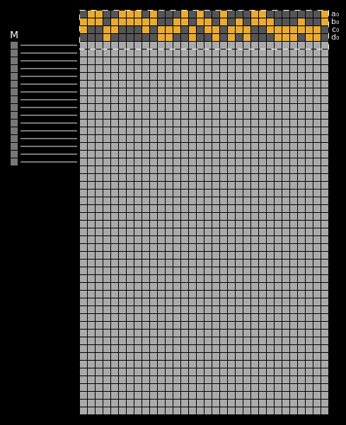
In that figure, the 32 bits of each intermediate MD4 state are represented across consecutive rows of the grid. You can see the order in which message words are mixed into the state. The dashed rectangle indicates which previous states are involved in computing the next state at any given step.

The final MD4 hash value is a function of the last four rows of this state grid. In other words, if two distinct inputs can produce the same values in these last four rows, those inputs will collide.

the structure of MD4 (in detail)

The previous section covered the concepts involved in computing MD4; the attack relies on those concepts, but it also relies on a number of (for lack of a better term) implementation details.

As a reference for these details, you can find my full implementation of MD4 here; within that codebase, all three rounds are calculated here. The most relevant aspects of the algorithm are also summarized below.

Let’s start by defining three simple boolean functions, \(F, G, H\). These are used by our round functions.

Trivial collisions exist for all three of these functions. The paper lists these on page 5:

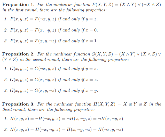
These collisions are important to the theory of the attack (though not to its implementation). For now, all you need to know is that \(F, G, H\) are used by the round functions \(r_1, r_2, r_3\) respectively.

Here’s what those round functions look like. As above, \(a, b, c, d\) are our four state variables. \(M = (m_0, m_1, ..., m_{15})\) is a fixed 512-bit message. \(k\) is an index into \(M\), and \(s\) is an amount to left-rotate by.

All additions are performed modulo \(2^{32}\).

In these definitions, \(\lll\) denotes the 32-bit left-rotate operation.

Within each of \(r_1\), \(r_2\), and \(r_3\), after the four state variables \(a, b, c, d\) are mixed together into a single value, the message word \(m[k]\) is added in (mod \(2^{32}\)) and the result is left-rotated.

Left-rotation and modulo addition are both invertable operations when one of their operands is known. This means that for any given arguments \(a, b, c, d, k, s\) and any desired result for the round, a simple algebraic method exists for determining a value of \(m_k\) which will produce that result. This gives us almost³ full control over the outputs of \(r_1\), \(r_2\), and \(r_3\).

Now, here’s how the round functions are applied to compute the hash function’s intermediate states.

# round 1
a = r1(a,b,c,d, 0,3,m); d = r1(d,a,b,c, 1,7,m); c = r1(c,d,a,b, 2,11,m); b = r1(b,c,d,a, 3,19,m)
a = r1(a,b,c,d, 4,3,m); d = r1(d,a,b,c, 5,7,m); c = r1(c,d,a,b, 6,11,m); b = r1(b,c,d,a, 7,19,m)
a = r1(a,b,c,d, 8,3,m); d = r1(d,a,b,c, 9,7,m); c = r1(c,d,a,b,10,11,m); b = r1(b,c,d,a,11,19,m)
a = r1(a,b,c,d,12,3,m); d = r1(d,a,b,c,13,7,m); c = r1(c,d,a,b,14,11,m); b = r1(b,c,d,a,15,19,m)

# round 2
a = r2(a,b,c,d,0,3,m); d = r2(d,a,b,c,4,5,m); c = r2(c,d,a,b, 8,9,m); b = r2(b,c,d,a,12,13,m)
a = r2(a,b,c,d,1,3,m); d = r2(d,a,b,c,5,5,m); c = r2(c,d,a,b, 9,9,m); b = r2(b,c,d,a,13,13,m)
a = r2(a,b,c,d,2,3,m); d = r2(d,a,b,c,6,5,m); c = r2(c,d,a,b,10,9,m); b = r2(b,c,d,a,14,13,m)
a = r2(a,b,c,d,3,3,m); d = r2(d,a,b,c,7,5,m); c = r2(c,d,a,b,11,9,m); b = r2(b,c,d,a,15,13,m)

# round 3
a = r3(a,b,c,d,0,3,m); d = r3(d,a,b,c, 8,9,m); c = r3(c,d,a,b,4,11,m); b = r3(b,c,d,a,12,15,m)
a = r3(a,b,c,d,2,3,m); d = r3(d,a,b,c,10,9,m); c = r3(c,d,a,b,6,11,m); b = r3(b,c,d,a,14,15,m)
a = r3(a,b,c,d,1,3,m); d = r3(d,a,b,c, 9,9,m); c = r3(c,d,a,b,5,11,m); b = r3(b,c,d,a,13,15,m)
a = r3(a,b,c,d,3,3,m); d = r3(d,a,b,c,11,9,m); c = r3(c,d,a,b,7,11,m); b = r3(b,c,d,a,15,15,m)

This code demonstrates a few important details of the algorithm’s design: first, the order in which previous intermediate states are passed to each invocation of the round function; second, the order in which message blocks are used in each round; third, the values of \(s\) used in each call to the round functions.

In the code block above, intermediate states are grouped into rows of four. Besides just looking nice, this mimics the paper’s notation. This notation denotes e.g. the first state on the first row as \(a_1\), the third state on the fourth row as \(c_4\), and so on. \(a_0, b_0, c_0, d_0\) denote the values to which the four state variables \(a, b, c, d\) are initialized.

The paper uses an extension of this notation to denote individual bits within states: for instance, \(c_{4,1}\) refers to \(c_4\)’s least significant bit, \(d_{2,14}\) refers to \(d_2\)’s 14th bit counting from the least significant end, \(b_{9,32}\) is \(b_9\)’s most significant bit (i.e. its 32nd-least significant bit), and so on.

This notation is important because it is used to express all of the paper’s constraints on MD4’s intermediate states. These constraints are central to the attack.

Note that by the paper’s convention, both subscripts here are 1-indexed rather than 0-indexed.

A quick note on terminology: The original paper prefers the term conditions over constraints when discussing the rules it defines for MD4’s intermediate states. Conditions is more in line with the attack’s theoretical underpinnings, but I feel that constraints is more reflective of how these rules are used when carrying out the attack. This post uses the two terms interchangeably.

defining the attack

The core of Wang’s attack is a large list of constraints on the hash function’s intermediate states. Despite what the paper says, these do not quite form a set of sufficient conditions, but they do come close. Here is the relevant table (from page 16 of the paper):

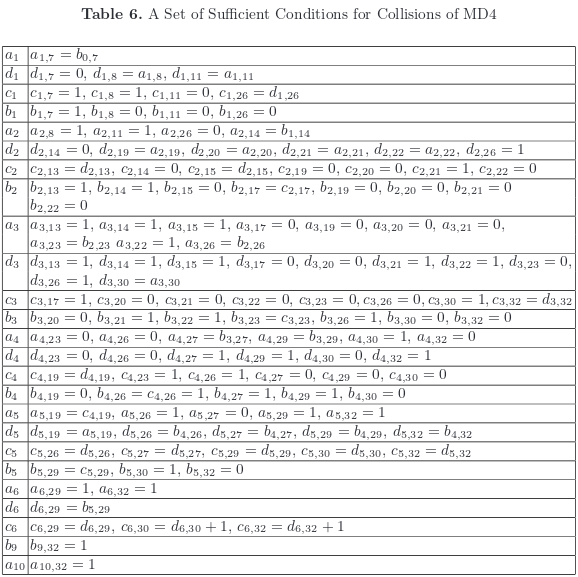
This may look like a lot, but if you stare at it for long enough you’ll start to notice patterns. Nearly all of the constraints fall into three broad categories: requiring that certain bits within intermediate states are either 0, 1, or equal to the bit at the same index in a prior state (almost always the immediately prior state). We can thus fit the bulk of these constraints into a three-part taxonomy: we have zero constraints, one constraints, and equality constraints. The only exceptions to this taxonomy are two constraints on \(c_6\), namely \(c_{6,30} = d_{6,30}+1\) and \(c_{6,32} = d_{6,32}+1\).

The bulk of these constraints apply to first-round intermediate states. According to Wang et al., satisfying the first-round constraints (i.e. everything up through \(b_4\)) is enough to produce a collision with probability \(2^{-25}\). If all the constraints are satisfied, then “the probability can be among \(2^{-6} \sim 2^{-2}\).” This sounds pretty good, but don’t get too excited just yet.

If I may editorialize for a moment: The fact that Wang et al. give such a broad range for the attack’s success rate (between 25% and 1.5%) may imply that they were unable to measure it directly, suggesting that even they did not have a full methodology for enforcing all of their conditions. They likely got close, but how close is anyone’s guess.

With that in mind, let’s see how close we can get.

The idea for the whole attack is something like this:

Generate a random input message; then, compute all the intermediate states generated by hashing this message; in the process of computing these states, derive and perform the message modifications necessary for these states to satisfy as many of the conditions from Table 6 as possible.

Wang et al. simply call this “message modification”, which is nice and alliterative but also a little generic. We can do better: let’s call this message modification method a message massage.

Massaging the message to satisfy some of Wang et al.’s conditions greatly increases the likelihood that \(H(m) = H(m + D)\). The more conditions satisfied, the higher the probability of success.

The next couple sections outline the message massage methodology. After that, we’ll take a look at the results of a successful massage.

massaging the message: round one

We’ll start with the message modifications needed to satisfy our round 1 conditions.

The process for these is straightforward: just start at the start and work down the list.

First, modify \(a_1\) so that the condition \(a_{1,7} = b_{0,7}\) is met. Then, derive the message chunk required to produce this modified \(a_1\). To do this, we need to solve the round function \(r_1\) for \(m_k\), like so:

If we know the value we want \(r_1\) to evaluate to, we can use this to find the message chunk which will produce that value. Let’s work through an example – here’s \(a_1\):

You can apply this just as easily for any other intermediate state, say \(c_3\):

It should be clear that this approach is applicable for each state in round 1, meaning that we can follow this process to make message modifications ensuring that all our conditions on \(a_1, d_1, c_1, ..., b_4\) are met.

Massaging the message to enforce all the round one conditions is enough to bring us to a success probability of roughly \(2^{-25}\). That’s not bad, but we can do better - at the cost of some added complexity.

massaging the message: \(a_5\)

One thing I’ve glossed over so far: whenever we change an intermediate state, this change has side effects on each subsequent intermediate state. For instance, changing \(c_3\) also implicitly changes \(b_3\), \(a_4\), \(d_4\), \(c_4\), \(b_4\), etc. Of course, the preceding states \(d_3\), \(a_3\), \(b_2\), \(c_2\), \(d_2\), etc, are all unchanged.

This is why our round one constraints have to be enforced in order: otherwise, they would run the risk of overwriting each other.

When we get to round two, our process for deriving a new \(m_k\) based on our desired modifications still works, but with a caveat: any change we make will propogates backward into round 1. For example, \(a_5\) depends on \(m_0\), but so does \(a_1\) – so if we modify \(m_0\) to enforce conditions on \(a_5\), we’ll end up changing \(a_1\) as well. This change will then propogate forward to \(d_1, c_1, b_1, a_2, b_2\), and so on, undoing all our hard work as it goes.

How can we prevent this? I’m glad you asked. Take a look at this diagram.

This illustrates the process of correcting a second-round state, \(a_5\). In this case, the process consists of three steps.

The first step is shown in the leftmost section of the diagram, where \(a_5\) is adjusted to meet our constraints and \(m_0\) is modified to produce the new value of \(a_5\). This change also alters the value of a previous state (\(a_1\)) and a later state (\(a_9\), omitted from this diagram).

We don’t really care if \(a_9\) changes, since we haven’t massaged that state.⁴ The change to \(a_1\), however, will have to be dealt with.

First, there is the possibility that our change to \(m_0\) modified \(a_1\) in such a way that our conditions on \(a_1\) are no longer satisfied. Some second-round conditions are more likely than others to mess up first-round conditions; for whatever reason, the conditions for \(a_5\) and \(a_1\) seem to coexist well.

If we were to find our first-round constraints invalidated by our second-round message massage, that would be a big problem. See the section on \(d_5\) for an example of one effective solution.

If the conditions on \(a_1\) are still satisfied, we can move on to the next step: containing the disruption caused by changing \(a_1\)’s value. This is illustrated in the middle section of the diagram. \(a_1\), shown in green, is in a known-good state; its direct dependencies \(d_1, c_1, b_1, a_2\) are highlighted in yellow to indicate that they have been disrupted by the change to \(a_1\).

Recall that we can derive the message modification necessary to set any intermediate state to any value (albeit not without side effects). If we’ve saved the old values of \(d_1, c_1, b_1, a_2\), we can just re-evaluate our equation with the new value of \(a_1\) to derive new message blocks \(m_2, m_3, m_4, m_5\) which will cause \(d_1, c_1, b_1, a_2\) to evaluate to their old values. Since these are \(a_1\)’s only direct dependencies, preventing them from changing prevents any further changes from propogating through round 1.

Of course, making these changes to \(m_2, m_3, m_4, m_5\) will create an even greater ripple effect, disrupting other states in round 2. This is shown in the third part of the diagram, where \(d_5, a_6, a_7, a_8\) are highlighted to show that their values have changed (changes to round 3 states are omitted to avoid clutter).

The critical thing here is that all of these states occur after the state we’re concerned with massaging (\(a_5\)). Thus we have managed to contain the impact from modifying \(a_5\) so that the only altered states are ones where no constraints have yet been enforced – meaning none of our work so far can be disrupted.

Well… almost none. There is still a chance of messing up our equality constraints. Take, for example, the constraint \(a_{2,14} = b_{1,14}\).

Suppose we update \(a_{2}\), and suppose further that we end up changing \(a_{2,19}\) in the process. Afterwards, as described above, we carefully make sure to preserve the old value of \(d_2\). Now, if \(a_{2,19} = d_{2,19}\) prior to these changes, then \(a_{2,19} \ne d_{2,19}\) afterwards. In other words, changing \(a_2\) has the potential to break our constraints on \(d_2\).

This can and will happen with many of our equality constraints, so whenever we modify a state that appears in another state’s equality constraints we have to make sure that these equalities still hold.

As it happens, our modifications to \(a_{2}\) don’t tend to disrupt \(a_{2,19}\). When we move on to massaging \(d_5\) and beyond, though, we will have to take this into consideration.

massaging the message: \(d_5\)

Moving right along: Our next task is to massage \(d_5\). This state takes \(m_4\) as input; \(m_4\) is also used by \(a_2\).

The considerations discussed above in the context of \(a_5\) apply here as well, but we have an additional challenge to overcome: our changes to \(d_5\) have a tendency to disrupt our earlier changes to \(a_2\). The reverse is true as well: if we re-massage \(a_2\), our changes are likely to break the constraints for \(d_5\). The method we have been using thus far to satisfy sets of constraints can get either \(a_2\) or \(d_5\) to a known-good state, but as long as we are enforcing these constraint sets separately, we are very unlikely to end up satisfying both of them at once.

There are several viable options here. My preferred solution is to combine the two sets of constraints. We will find a way of translating them from constraints on states to constraints on the corresponding message word from which those states are derived. This requires some careful bookkeeping, but it will allow us to enforce both sets of constraints simultaneously, preventing them from conflicting with each other.

Recall that the round functions \(r_1, r_2\) are defined like so:

The values of \(a, b, c, d\) come from previous states, so within any individual state calculation we can take these values as constant. This allows us to simplify the round functions somewhat. We’ll start by consolidating the round functions’ constant terms; this will allow us to clean up the formulae for our intermediate states:

Through these final equalities, we can translate constraints on \(a_2\) and \(d_5\) into constraints on \(N_1 + m_4\) and \(N_2 + m_4\) respectively.

We will adapt our earlier notation to denote specific bits within these sums, e.g. \((N_2 + m_4)_5\) for the 5th bit of \(N_2 + m_4\).

Take the constraint \(a_{2,8} = 1\). We can translate this as \((N_1 + m_{4})_5 = 1\). Note that the original constraint’s index of 8 becomes 5 after translation. Indices of \(a_2\)’s constraints need to be adjusted by 3, as shown; indices for \(d_5\)’s constraints need to be adjusted by 5. This is to compensate for the round functions’ bit rotations. The rest of the translation process is pretty simple.

The full list of translated constraints is as follows.

As luck would have it, all of these constraints apply to distinct indices. If this were not the case, then we would have a bit of an awkward situation,⁵ but as things stand it is straightforward to enforce all of these at once.

Our general methodology will be to work from low-order bits upward. For each bit, we will note the value it has and the value we want it to have. If the constraint is already satisfied, we do nothing; otherwise, we flip the corresponding bit in \(m_4\). Since addition is just xor with carries, this will suffice to flip the bit in the sum. Note that this modification also has the potential to modify higher-order bits in the sum, meaning we will have to re-evaluate the sum after each modification to \(m_4\).

After making the necessary changes to \(m_4\), we will need to update \(m_5\) thru \(m_9\) to contain those changes’ side effects. We will also want to re-massage \(d_2\) to ensure that its equality constraints with \(a_2\) are still met.

This method allows us to satisfy all of \(d_5\)’s constraints.

It is possible to massage the state further, but each further step adds new complications and this post is already getting long.

tracking the state differential

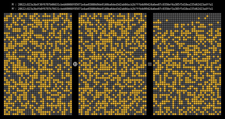
In order to see if our collision is working, we look at the xor difference of the two messages’ intermediate hash states. This shows us where state differentials are introduced, as well as (hopefully) where they disappear.

Recall that MD4’s final result is computed from the last four internal states; as a corollary, if the last four rows of two messages’ state differential are all 0 then those two messages form a collision.

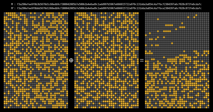
Here are the state differentials for one hundred random messages (hover to animate):

You can see exactly where the first message differentials are introduced, and the resulting state differential, in the second and third rows of round one. These early divergences quickly compound on themselves, and soon the differential has diffused throughout the entire state.

Here are the state differentials for one hundred moderately massaged messages (again, hover to animate):

And finally, here are the state differentials for one hundred collisions (hover):

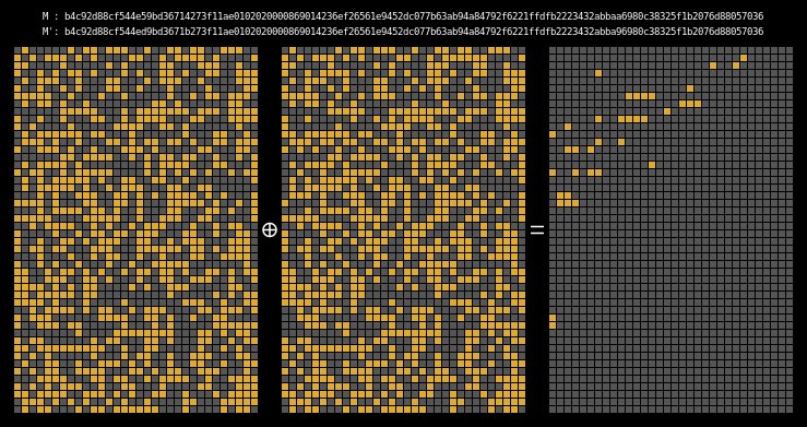
Recall that we showed earlier that two messages will collide when their state grids’ last four rows have a differential of 0. We can see that this is indeed the case for all of our colliding messages.

The paper states (on page 7) that it is clear that the collision differential consists of two internal collisions respectively from 2-25 steps and 36-41 steps. I think it’s kind of cool how the above graphic allows us to visually confirm this.

I haven’t gone through the whole process of proving these internal collisions’ validity, but if I were to do so my proof strategy would make heavy use of the boolean function collisions described above, since those give you conditions under which any round’s differentials will fail to propogate forward.

countermeasures

You may be wondering how modern hash functions defend against this sort of attack. Well, there’s a long answer and a short answer. The long answer could fill a book; the short answer is that modern designs take greater pains to ensure dispersion of differentials through the function’s full internal state.

For instance, SHA-1 and SHA-2 use “message expansion” steps which expand the 16 words of a message block into input buffers of 80 or 64 words respectively. In both cases, the expansion step is designed so that changing any of the 16 message chunks will result in a large number of changes throughout the expanded message. Message expansion takes place before the (expanded) message is mixed into the hash function’s internal state. As a consequence, any small change to the message will produce many more (and more complex) changes to the internal state than in MD4.⁶

Another defense is to simply build a hash function around something other than the Merkle-Damgård construction; a good example here is SHA-3, which uses a radically different design based around a sponge function.

By definition, sponge function must provide effective dispersion of differentials in order for sponge constructions to work. This is nontrivial to ensure, but the resulting algorithms are strikingly simple and comes with elegant security proofs. I’m no expert, but reading about SHA-3 and sponge constructions makes me wonder why we haven’t been building hash functions this way all along.

conclusion

That just about does it for the theory behind Wang’s attack. Tune in next time for a discussion of how the attack might be implemented cleanly and efficiently in Python.