sohliloquies
A New Method for Estimating P2P Network Size
5 June 2020Background
Every member of a DHT network knows about their immediate neighbors, but no one has a full view of the network state. So, how can we measure network size?
I’m going to focus on Kademlia-style networks in this post. Most big DHTs are based on Kademlia. Other DHTs with similar routing properties might be able to adapt this methodology.
Previous work on estimating the size of Kademlia-based DHTs has focused on “walking” subregions of the address space. The idea is to count the number of nodes found in some arbitrary interval, then to scale that up to provide a size estimate for the full network.1
This idea seems simple enough, but it turns out to contain a subtle flaw. Even if peer density is uniform, there is still the problem of measuring peer density accurately. Any walk over a region of the address space is going to miss some peers; this, if not compensated for, will lead to an underestimate of the actual peer density, which in turn will lead to an underestimate of network size.
This page does a good job of discussing this issue. Incredibly, they show that deriving a size estimate from a naive walk leads to “errors on the order of tens of percents”. Their proposed solution is: measure the probability of any given peer being missed by a walk through the address space, then to use this probability to derive a “correction factor” by which their peer count is adjusted. This tries to compensate for however many peers they assume they missed. The results sound accurate, and they claim this technique can produce a size estimate “in about 5 seconds”.
They do not mention how many address lookups the process requires. However, looking at their code and their published results, we can guess that it is likely on the order of tens of thousands of queries.2
I’d like to share a simpler methodology that is based on ordinary address lookups. These lookups can be performed in parallel and they can be for arbitrary addresses. This means that not only can size estimates be produced very quickly, but they can also be produced as a byproduct of ordinary network activity.
The Idea
Let’s start from first principles. The network consists of nodes. Each node has a node ID. Node IDs are random bitstrings of length \(L\). Thus, node IDs are evenly3 distributed through an address space of size \(2^L\). Distance between addresses is measured with the XOR metric.
Let \(n\) be the number of nodes in the network. We don’t know the value of \(n\) yet, but we’ll get to that.
Choose an arbitrary address \(A\). What is each node ID’s distance from that address? We can compute these with a curried XOR: \(f(I) = I \oplus A\).
\(f\) defines a bijective map from the address space to itself. We’ll define \(D = \{D_1, \ldots, D_n\}\) as the image of our node ID set under \(f\).
For convenience, let’s consider these distances not as bitstrings but as integers on the range \([0, 2^L-1]\), and let’s specify (without loss of generality) that \(D_1 < D_2 < \ldots < D_n\).
Under these definitions, \(D_i\) is precisely the \(i\)‘th order statistic of \(D\).
Discrete random variables’ order statistics are a pain to analyze, but it turns out we can get away with simplifying things by swapping out our discrete random variables for continuous ones. This adds only a negligible error term.
If we approximate \(D_1, \ldots, D_n\) by the order statistics, in order, of a sample of \(n\) uniform random variables, and we normalize these variables from \([0, 2^L-1]\) to \([0, 1]\), we end up with \(n\) new random variables \(N = \{N_1, ..., N_n\}\) where \(N_i \approx \frac{D_i}{2^L-1}\).
These normalized random variables \(N_i\) can be shown to follow specific beta distributions. The parameterization is \(\alpha = i, \beta = n - i + 1\), and the derivation is on Wikipedia. The beta distribution’s mean under this parameterization is \(\operatorname{E}[N_i] = \frac{i}{n+1}\).
See where I’m going with this? We can just rewrite \(\operatorname{E}[N_i] = \frac{i}{n+1}\) as \(n = \frac{i}{\operatorname{E}[N_i]} - 1\).
Size-\(k\) lookups allow us to sample \(N_1\) through \(N_k\). Running multiple lookups in parallel allows us to take averages across (effectively) independent samples for each of \(N_1, \ldots, N_k\).
As long as these lookups are not too tightly clustered, then by the central limit theorem we can expect the distributions our averaged measurements for \(N_1, \ldots, N_k\) to converge to normal as the number of lookups increases.
Each one of those variables can be plugged into the given equation to produce a network size estimate. Individual size estimates are somewhat noisy, but they can be combined to provide a stable, accurate estimate for the value of \(n\).
The naive way to combine these estimates would be to take their average. With a little more work we can instead compute a least-squares fit to find a value of \(n\) which minimizes error terms across all our sampled values \(N_1\) through \(N_k\). The derivation is nothing special but I’ll include it for the sake of completeness. Our least-squares error function is:
\[e(n) = \sum\limits_{i=1}^{k}(N_i - \frac{i}{n+1})^2\]We’ll minimize this by setting the derivative equal to zero and solving.
\[\begin{align} \frac{de}{dn} &= \sum\limits_{i=1}^{k} \frac{2i(n N_i + N_i - i)}{(n+1)^3} \\ &= \frac{2}{(n+1)^3} ((n+1) \sum\limits_{i=1}^{k} i N_i - \sum\limits_{i=1}^{k} i^2) = 0 \end{align}\]After simplifying and applying an identity for \(\sum\limits_{i=1}^{k} i^2\), we get the following:
\[\begin{align} (n+1) \sum\limits_{i=1}^{k} i N_i &= \frac{k(k+1)(2k+1)}{6} \\ \\ n &= \frac{k(k+1)(2k+1)}{6 \sum\limits_{i=1}^{k} i N_i} - 1 \end{align}\]This final equation can be transcribed directly into code and evaluted. Here are Python implementations for both of the size estimation methods I’ve described.
k = 8   # fixed, globally known network parameter


def avg_est(D_i):  # naive method
    return sum(i/d - 1 for i, d in enumerate(D_i, 1)) / k


LSQ_CONST = k*(k+1)*(2*k+1) / 6   # we can precompute this since k is constant


def lsq_est(D_i):  # least-squares method
    return LSQ_CONST / sum(i*d for i, d in enumerate(D_i, 1)) - 1
Both methods are accurate, but the least-squares method turns out to be somewhat more precise.
By increasing our sample size we can get arbitrarily accurate estimates for network size. Since lookups can be computed in parallel, we can increase the estimate’s accuracy without slowing it down at all.
Experimental Validation
OK, that sounds too easy, right? Let’s check our math by running some tests on simulated networks. The goal here is to see if our statistical models predict these simulations’ behavior correctly.
Here are measurements for the distributions of \(N_1\) through \(N_8\) for a network with \(n = 1000\) peers. The model’s predicted beta distributions are superimposed in orange.

Here is a version of that same chart for a network with very few peers (\(n = 10\)):

And here is \(n = 100{,}000\).
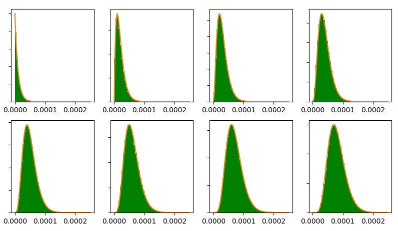
Smaller networks can be seen to lead to noisier (though not inaccurate) measurements. For large networks, the distribution is matched just about perfectly.
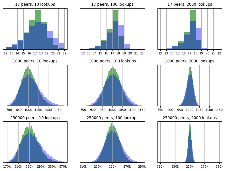
The next step is to combine these measurements into an overall size estimate. There are many reasonable ways to do this. I’ve illustrated the results of two simple ideas on a variety of networks below.
These charts are histograms showing many independent size estimates on many different networks of a given size. If it helps, you can think of these as approximating probability density functions for size estimates under the given parameterizations.
Being histograms, the y-axis shows relative frequency, which is why I’ve left it unlabeled: columns’ values in terms of any absolute units would just end up being a function of the sample size and bucket sizes and would not convey anything useful.
Both methods start by taking unweighted averages across all the measurements for each order statistic. The blue curve shows the result of generating a size estimate from each measurement and then averaging those estimates. The green curve shows the result of deriving the estimate from a least-squares fit (as discussed in the last section).
Some hardcore stats nerd could probably find an even more accurate method for generating consolidated size estimates; if that’s you, I’d love to hear about it.
If you’re interested in the code that generated these figures, see here.
Here are the 95% confidence intervals for the green curves in the charts above.
| n | 10 lookups | 100 lookups | 2000 lookups |
|---|---|---|---|
| 17 | 17.2 ± 20.67% | 17.1 ± 12.41% | 17.1 ± 11.24% |
| 1000 | 1015.9 ± 23.53% | 1002.5 ± 7.71% | 1000.0 ± 3.11% |
| 250k | 253741.4 ± 23.67% | 250479.2 ± 7.40% | 250192.5 ± 1.66% |
Discussion
Both methods of consolidating size estimates can be seen to produce fairly accurate results. The least-squares method is more precise in all cases.
The size estimates’ distribution is somewhat asymmetric; as a result, each estimate’s distribution’s mean slightly exceeds its mode (as can be seen above - the samples’ modes consistently align with the correct size estimates, while their means – listed in the table – tends to slightly exceed it).
Averages over large numbers of lookups seem to converge to the normal distribution. This is a straightforward consequence of the central limit theorem. This implies that while the estimates’ distribution may be asymmetric, the distribution to which it converges is symmetric, and thus the distribution’s mean eventually does converge with its mode.
The technique seems to work much better on large networks than on small ones. Note in particular how in the “100 lookups” and “2000 lookups” columns in the table above, the error percentages monotonically decrease as network size increases. This suggests that for a sufficiently large, fixed number of queries, increasing the network size measurably improves this method’s accuracy. This makes sense: the intuition is that inserting more evenly distributed node IDs reduces the variances of our distance variables, thus lowering the amount of noise in our estimate.
For very small networks, it may be just as effective to produce size estimates through traditional methods. However, for networks of any substantial size, the method given here is likely to be faster and more accurate.
Detecting Sybil Attacks
It turns out that once we have a network size estimate, we also get Sybil attack detection for free.4
Real-World Sybil Attacks in BitTorrent Mainline DHT (PDF) gives a taxonomy sorting Sybil attacks into three categories: “horizontal”, “vertical”, and “hybrid”. Horizontal attacks target the entire network; vertical attacks target specific addresses; hybrid attacks are a mix of both methods.
For a Sybil attack on a specific address to be successful, the attacker needs lookups for that address to yield only attacker-controlled peers. This means subverting the routing overlay and/or simply outnumbering honest peers by a massive margin.
Attacking the routing overlay requires a large-scale horizontal or hybrid attack; these are easy to detect because they register as a massive increase in network size (likely combined with a decline in the network’s usefulness). If every peer is passively maintaining an accurate estimate of network size at all times then such an event could hardly go unnoticed. The best defense is simply to deploy more honest peers on the network.
What about vertical Sybil attacks? These are harder to passively detect, because they are entirely localized around a target address. This is also the key to detecting them. These attacks can only succeed if the attacker controls the \(k\) closest nodes to the target address, which means deploying at least \(k\) Sybil nodes closer to the target address than the closest honest peer.
The closest honest peer’s expected distance from an arbitrary address is \(\operatorname{E}[D_{1}]\). If a (successful) vertical Sybil attack is underway, we will observe that \(D_{k} > \operatorname{E}[D_1]\). The probability of this happening by random chance is extremely low.5 In fact, it is low enough that the test is still reliable even when our estimate of network size is still noisy.
Thus, once we have an up-to-date estimate of network size, we also have an extremely reliable test for whether any given address is the target of a vertical Sybil attack. The cost of this test is one lookup for the target address, meaning we can simply run it on every lookup we perform.6
Conclusion
This passive method for measuring DHT network size greatly lowers the cost of tracking some basic network metrics; it also allows us to detect (and possibly respond to) Sybil attacks on the network.
I shared the results of – and the source code for – a thorough experimental validation of this methodology. There is almost certainly room for improvements, and there are likely some wrinkles to iron out; however, it is clear that the core idea is both practical and effective.
Perhaps surprisingly, the method is shown to work much better on large networks than small ones, and to increase in accuracy monotonically as network size increases.
Everything described here relies only on ordinary lookups for arbitrary addresses, meaning size estimates can be produced as a byproduct of ordinary network activity. This allows peers to maintain up-to-date estimates of network size essentially for free.
This is original research. I could not find any prior published descriptions of this method, and it is several orders of magnitude faster than the next-best published methodology of which I am aware.
-
Note that this relies on the assumption that peers are evenly distributed through the address space. See here3 for more on this. ↩
-
Reviewing their published code, it appears that their walker sends five lookup queries to each node it finds in the target subregion, and one query to each node it finds outside that region. They use a “12-bit zone”, and Fig. 2 from their published paper suggests that such a zone can be expected to contain roughly 5000 nodes. It seems reasonable to expect that something roughly on the order of 25000 queries might be sent over the course of the crawl. Note that this count does not include the queries required to produce an experimental measurement for the “correction factor”. ↩
-
Technically, Kademlia does not require even distribution, and some DHTs like MLDHT allow nodes to choose their own IDs. About this, the authors of the paper linked above write, “we carefully examined a large set of samples (over 32000) crawled from the different parts of MLDHT, and found the node IDs follow a uniform distribution. We did observe some abused IDs such as ID 0, but they only contribute a trivial amount of nodes to the whole MLDHT, and can be safely neglected in our case.” Some variants of Kademlia further encourage even distribution of nodes through the use of a cryptographically secure hash function. ↩ ↩2
-
Sybil attacks are notoriously hard to defend against. Note that this does not necessarily mean they are hard to detect; the difference between detection and defense is something like that between diagnosis and cure. Perfect defense against Sybil attacks is not possible in a fully ad-hoc setting; however, we can take some steps to limit their impact. See footnote6 for more on this. ↩
-
If we assume that all node IDs (including Sybil IDs) are uniformly distributed, then the probability \(P(D_{k} > \operatorname{E}[D_1])\) is just given by the CDF of \(D_k\) at \(x = \operatorname{E}[D_1]\). The precise value varies with network size and parameterization but it can be expected to be extremely small. On the other hand, if node ID uniformity is not enforced, then the attacker can simply measure \(D_1\) and hope that its actual value exceeds \(\operatorname{E}[D_1]\) – in which case they can fool our simple test. There might be other tests (perhaps involving \(D_{1}, \ldots, D_{k-1}\)) which would be harder to fool; investigating these is left as an exercise for the reader. ↩
-
Taking this idea a step further: once we have a method for detecting vertical Sybil attacks, we can start to consider ways that the network might adapt around these attacks. What if, whenever a peer’s lookup detected a vertical Sybil attack, they knew to expand that lookup’s result set? And what if peers noticed when vertical Sybil attacks were taking place at addresses close to their own node IDs and were more generous with storage durations for data stored at those addresses? This, combined with the use of a hash function for node ID assignment, could go a long way towards neutralizing vertical Sybil attacks. ↩ ↩2