Introduction

This post discusses some well-known security issues with modern distributed hash tables.

We start with a discussion of attempted solutions, then review the current best-known solutions. Some issues with these are identified and discussed, and remediations are proposed. The final section, which makes up the bulk of the post, consists of a thorough mathematical analysis of these remediations’ effectiveness.

It is shown that while Sybil attacks cannot be prevented entirely, they can be made impractical while introducing only negligible overhead for honest peers.

This post’s main contribution is a method for quantifying precisely how impractical a Sybil attack may be under any given set of network parameters. The results are surprisingly strong, and indicate some very easy and simple design changes that could greatly increase the security margins of modern DHTs.

Background

Sybil attacks are really hard to defend against. The basic issue is this: if you have a peer-to-peer network that anyone can join anonymously, there’s no good way to keep someone from joining a bunch of times under a bunch of different identities. An increased presence in the network often leads to an outsided level of influence over it; this is the root of the problem.

I’ll take a moment to summarize the conclusions of some surveys¹ on the subject.

The simplest and most common solution is to introduce a central authority who certifies identities. This solution has been breathlessly proposed many times. Of course, it completely sacrifices decentralization and anonymity, and so it is not appropriate for ad-hoc peer-to-peer settings.

OK, so that’s a no-go – what else has been tried?

A couple other common solutions: associating identity with some invariant aspect of network topology, or associating it with social graph data. The former of these is fragile and inflexible,² and the latter compromises user privacy by design. These compromises are clearly are not acceptable either.

The fourth solution class, and the one that has seen the most interesting results in ad-hoc contexts so far,³ is proof-of-work. It has been proposed that peers could periodically send puzzles to each other, the idea being that if a peer can’t promptly find and send a solution, they are not to be trusted. This places an upkeep cost on each identity operated, thus theoretically pegging an attacker’s total number of identities to their computational capacity.

This is an improvement: we aren’t leaking any social metadata, we aren’t relying on anything fragile (as far as we know), and we need no central authority. However, there are drawbacks: First, the overhead for this scheme is very high,⁴ and second, it penalizes peers for maintaining connections with a large number of peers (since this will result in them receiving more challenges). This disincentivizes broad engagement with the network. These drawbacks are also serious, and they are hard to avoid in the general case.

The above is just a quick overview geared towards giving you some idea of the main sorts of proposed solutions; for some more thorough surveys, see the footnote.¹

Proof-of-Work Kinda Works

The 2002 paper which introduced the term “Sybil attack” also proved that “without a logically centralized authority, Sybil attacks are always possible except under extreme and unrealistic assumptions of resource parity and coordination among entities.”⁵

It has been shown, then, that the attack cannot be defended against in general. However, its impact can be mitigated in specific cases.

The classic success story (if we can call it that) is Bitcoin; for all that Bitcoin is tremendously wasteful, it also actually no-shit works. We take it for granted today, but a decade ago this was flat-out miraculous.

The reason Bitcoin works is because peers gain influence in the network by solving proof-of-work problems. Thus, your influence is constrained by the amount of compute power you can afford to bring to bear.⁶

The problem, of course, is that Bitcoin’s security is predicated on the combined hash rate of all honest peers exceeding that of any attacker. Thus, honest peers must pay greater hardware and power costs than any attacker can afford to – at all times. Bitcoin’s security assumption might be stated as: none of us can afford to be as wasteful as all of us.⁷

Anyway, the point of that digression was to set up this question: we’ve seen that proof-of-work works, but can it work efficiently? I believe that it can. I’d like to describe an idea, and provide some analysis for it, in the specific context of distributed hash tables. First, though, we’ll need a little more background.

Kademlia and S/Kademlia

Let’s talk distributed hash tables. All sorts of DHT designs are proven to work in theory, but in practice Kademlia is the most popular by far. If you’re not already familiar, Wikipedia has a good article that you might want to scan through before continuing.

Plain Kademlia (as implemented in e.g. Mainline DHT) is horribly insecure. The currently recognized state of the art (as far as I’m aware) is a variant called S/Kademlia.⁸ You can tell S/Kademlia is an improvement because it has “S”, which stands for Secure, in the name.⁹

How secure is it?

Let me first say: The S/Kademlia designers have some really good ideas. They provide interesting and compelling modifications to the stock peer lookup algorithm. I consider that to be the best part of their work. They also recognize the need to prevent peers from choosing their own Node IDs, which is simple but very important.

They propose generating node IDs from cryptographic hashes of identity-certifying public keys. These keys are used for authentication and to ensure message integrity. For Sybil defense, two options are provided.

First, they suggest that public keys could be endorsed by a central authority. We have already discussed and dismissed this option.

Second, they suggest sharing public keys alongside solved computational puzzles. This is similar, but not identical, to the fourth solution class discussed earlier: the differences are that peers come up with their own puzzles (instead of being challenged), and the puzzle only has to be solved once, when the peer is first initialized, rather than on an ongoing basis.

Unfortunately, one of the puzzles specified in the S/Kademlia paper is broken.

Breaking S/Kademlia

If this were a Wikipedia article, this would be the part where you’d see a giant red banner saying something about “WARNING: ORIGINAL RESEARCH.” Let’s just acknowledge that up front.

Now, here are the two puzzles given for S/Kademlia. A peer needs to solve both for their node ID to be accepted.

Let us define the following: a cryptographic hash function \(H\), a method for generating public/private keypairs \(s_{\text{pub}}, s_{\text{priv}}\), and a pair of constant integer parameters \(c_1, c_2\) (which allow us to tune the difficulties of the first and second puzzles respectively).

Now, first, here is the “static” puzzle:¹⁰

1. Generate a keypair \(s_{\text{pub}}, s_{\text{priv}}\).

2. Calculate \(P := H(H(s_{\text{pub}}))\).

3. If any of the first \(c\) bits of \(P\) are not 0, goto 1.

4. The node ID is \(H(s_{\text{pub}})\).

There are several drawbacks to this scheme. It considers any given public key to be either valid or invalid, with the majority of public keys being invalid. Constraining the set of valid keys like this opens up some trivial theoretic attacks.¹¹ Pre-existing identity keys generally can’t be imported since the great majority of them will not pass validation. The scheme also requires two hash function evaluations when really only one should be necessary.

Now, here is the second, “dynamic” puzzle:¹²

1. Import \(\text{NodeID}\) from the previous problem.

2. Choose a random X.

3. Calculate \(P := H(\text{NodeID} \oplus X)\).

4. If any of the first \(c\) bits of \(P\) are not 0, goto 2.

5. This puzzle’s solution is \((\text{NodeID}, X)\).

The paper claims that the dynamic puzzle “ensures that it is complex to generate a huge amount of nodeIds”. It is then stated that “crypto puzzle creation has \(O(2^{c_1} + 2^{c_2})\) complexity”. For a naive attack these values are certainly correct.

The issue is that once an attacker has identified any hash input \(I\) which passes the puzzle’s test, they can set X to produce that input: \(X := \text{NodeID} \oplus I\). This works since there is no way for remote peers to verify that X is truly random.

Thus, once a suitable value \(I\) has been found,¹³ additional solutions to the second puzzle may be generated for free, lowering the total complexity to \(O(2^{c_1})\), the cost for the first puzzle.

Fixing S/Kademlia

A trivial mitigation would be to swap out XOR for concatenation in the dynamic puzzle. This would just mean redefining step 3 in puzzle 2 to read, \(P := H(\text{NodeID} \vert X)\). An alternative would be to use a more robust construction like \(P := \operatorname{HMAC}(\text{NodeID}, X)\). This would work, but stay tuned to see how we can do even better.

Of course, it bears mentioning that either of these would be breaking changes… but perhaps breaking backwards compatibility with a broken system is not such a bad thing.

Another note: The paper does not specify that \(H\) should be a hard function, only that it should be cryptographically secure; however, most classic cryptographic hash functions are specifically tuned for speed, making them unsuitable for use in proof-of-work constructions. Common sense dictates that a hard function should be used for \(H\). I’d suggest a modern, x86-optimized, memory-hard password hashing function like Argon2.¹⁴

If we are using a hard function for \(H\), then we need to pay attention to how many calls we’re making to this function in order to verify a remote peer’s NodeID. S/Kademlia’s two-puzzle construction requires three calls: one to generate the NodeID, one more to check the static puzzle, and a third one to check the dynamic puzzle. We can improve on this.

Argon2 allows us to generate arbitrary-length hashes. Say NodeIDs are 20 bytes long (as in the Kademlia specification). We can simply parameterize \(H\) to generate hashes of byte-length \(20 + \lceil \frac{c_2}{8} \rceil\), then treat the first 20 bytes as the NodeID and apply our proof-of-work test to the following \(c_2\) bits.

This allows us to get the strengths of both puzzles (NodeIDs determined by hash function, node generation constrained by puzzle with tunable difficulty level) while improving validation speed by a factor of three.

Another improvement: Why should nodes only have one ID? If your available RAM greatly exceeds the amount of data people want to store near your node ID (as is almost certainly the case in the year 2020) then really you’re letting resources go to waste by only claiming responsibility for that one neighborhood. Why not claim as many IDs as you can reasonably support?

If we’re still including an arbitrary value X in the node ID generation hash, then there’s no reason not to allow peers to just provide several values of X and to let them claim all the corresponding node IDs. If Sybil attackers are running multiple nodes on the network, why not let honest peers do the same thing?¹⁵

Note also that using a hard function for \(H\) allows us to get by with much smaller values for our work constant \(c\). Since our trial rate will be dramatically reduced, our trial success probability can afford to dramatically increase.¹⁶

This, in turn, allows us to consider doing more with X. What if X wasn’t arbitrary? What if we gave it some form of significance? Increasing our success probability means we’ll have to try fewer values of X to find a solution, so we can certainly get away with adding some semantic significance to X.

Bear with me: what if we treat it as an expiration date? That is, we’d predefine a window of validity (say 36 hours), and we’d only accept NodeIDs if their corresponding values of X represented Unix timestamps between now and 36 hours from now.¹⁷

This changes the cost equation for both attackers and defenders.

On the defenders’ side, honest peers have to solve puzzles once every couple days¹⁸ rather than solving only a single puzzle when they first join the network.

On the attackers’ side, it is no longer to generate a huge number of Sybil NodeIDs; now, they have to generate that many every 36 hours. Instead of requiring an attacker to compute some large total number of hashes, we’re now them to be able to field a large, sustained hash rate.¹⁹

Since attackers have to solve the proof-of-work problem many more times than defenders in order to be effective, this change to the cost equation has a significantly greater impact on attackers than defenders.

How much of an impact? I’m so glad you asked.

Modeling Sybil Attacks on S/Kademlia and Related Networks

If you thought the last sections were heavy on original research… buckle up.

I arrived at the following as part of my research for the Theseus DHT project (which is currently on indefinite hiatus). I’ve been sitting on this result since 2018; I was waiting until that project was further along before writing this up, but it’s looking like that won’t happen soon, so I guess I’ve waited long enough.

A couple years ago I did a fairly thorough literature review and was not able to find any prior art for the model I’m about to share. Now, I’m no academic, I don’t happen to know any subject matter experts to consult with on this, and I haven’t done any lit review since that survey a couple years ago; all that being said, to the best of my knowledge this is the first time the following work has been published. If you know of any prior art, please send it my way.

Definitions

Let’s start with some constants.

Let \(L\) denote the length of node IDs (in bits). In S/Kademlia, \(L = 160\). Some other Kademlia-based DHTs set \(L = 128\). Either value is fine.

Let \(n\) denote the number of honest nodes on the network at some moment in time.

Let \(m\) denote the number of malicious (i.e. Sybil) nodes on the network at the same moment.

Let \(k\) denote the size of our routing lookup sets.

We will be dealing with a number of random variables following the hypergeometric distribution; for these, we will write \(X_{p,s,d}\) where \(p_{}, s, d\) denote the population size, number of success states in the population, and number of draws from the population (without replacement), respectively.

Network Model

The Kademlia address space may be thought of as a binary tree of height \(L\), structured as a prefix tree, with each leaf representing an address (or, equivalently, a node ID, since both are length-\(L\) bitstrings).²⁰

Note that as a straightforward consequence of the XOR metric’s definition, any leaf in a given subtree will be closer to any other leaf in that subtree than to any leaf outside it.

With regard to node IDs, each leaf in the tree may be considered as being in one of three states: unoccupied, honest, or Sybil, depending on whether the corresponding node ID has been claimed (and by whom).

With regard to data addresses, we may consider each leaf to be in one of two states: compromised or resilient, depending on whether a lookup for that data address would return at least one honest node (i.e. whether the network’s redundancy factor \(k\) is sufficient to maintain the integrity of any data stored at the given address).²¹

Collocation

Some notes on collocation: First, we know that honest nodes are evenly distributed through the network, since their distribution is determined by a cryptographically secure hash function. As a result, accidental node collocation between honest peers is extremely unlikely. Modeling this as an instance of the birthday problem, the probability would seem to be negligible until the number of honest nodes is at least on the order of \(10^{19}\) for \(L = 128\) or \(10^{24}\) for \(L = 160\). For scale, Earth’s total population is currently below \(10^{10}\).

Collocation between honest and malicious peers is also exceedingly unlikely, though not strictly impossible. An attacker with truly massive compute power might sometimes be able to cause this to happen as part of a vertical Sybil attack.²²

Handling this edge case requires a minor alteration to our lookup logic: rather than looking up \(k\) peers, let us cut off our lookups once we’ve found at least \(k\) peers and \(k\) IDs. The distinction may seem insignificant, and in practice it almost always will be, but it is of theoretic significance because it allows us to say that whenever a honest and a malicious peer collocate, the corresponding leaf node is considered honest.

Terminology

Here are some higher-level concepts based on the ideas we’ve just discussed. This will feel dense; I apologize. For what it’s worth, these definitions make the following derivations much easier to follow.

A non-empty subtree (or NEST) is a subtree containing at least one honest node.

An empty subtree (or EST) is a subtree containing only unoccupied or Sybil nodes.

A maximal EST is a subtree which is an EST but whose parent (if it has one) does not have the same property.

Equivalently: a maximal EST is an EST whose sibling is a NEST (or which has no sibling, if it is the root of the tree, as would occur in the degenerate case of a network composed only of Sybils).

The resilience coefficient for a subtree of height \(h\), denoted by \(R_{h,k}\), is a value on the range \([0, 1]\) denoting the ratio of resilient nodes to total nodes in the subtree with lookups of size \(k\).

Note that \(\operatorname{E}[R_{h,k}]\) will be equal for all subtrees of any given height \(h\), since the tree’s structure is symmetric and even node distribution preserves this symmetry.

Let \(A_{h,x}\) denote the event of a height-\(h\) subtree containing precisely \(x\) Sybil nodes (attackers).

Let \(D_{h,x}\) denote the analogous event of a height-\(h\) subtree containing precisely \(x\) honest nodes (defenders).

Let \(N_h\) denote the event of a height-\(h\) subtree being a NEST. \(N_h = \lnot D_{h,0}\) by definition.

Let \(E_h\) denote the event of a height-\(h\) subtree being a maximal EST. \(E_h = N_{h+1} \land \lnot N_{h}\) by definition.

Bitstrings will be indicated by a subscripted \(b\), like so: \(10101_b\). Note that in bitstrings, unlike ordinary numbers, leading zeroes have semantic significance.

Example: Evaluating a Prefix Tree

This illustration shows a simple toy network with \(L = 5, a = 5, d = 5\).

Each leaf represents an address (or node ID) determined by the leaf’s position in the prefix tree. Starting from the left, we have \(\text{00000}_b\), \(\text{00001}_b\), \(\text{00010}_b\), \(\text{00011}_b\), etc.

The green leaves represent honest peers and the red leaves represent Sybil peers.

Under the tree, we have three rows. These represent the states of the leaves’ data addresses for \(k \in \{1, 2, 3\}\). You can see that each address is either resilient (green) or compromised (red), and that the number of resilient addresses rises sharply as \(k\) increases. Note that real networks use much larger values of \(k\), e.g. \(k = 8\) or \(k = 16\).

You can mouse over any address in these last three rows to see which peers are included in its size-\(k\) lookup set.

Let’s use this figure to help review our terminology.

The honest nodes are \(\text{00001}_b\), \(\text{01001}_b\), \(\text{01010}_b\), \(\text{01111}_b\), and \(\text{10001}_b\).

The Sybil nodes are \(\text{00110}_b\), \(\text{01101}_b\), \(\text{10010}_b\), \(\text{10100}_b\), and \(\text{10111}_b\).

The maximal ESTs’ root nodes are \(\text{00000}_b\), \(\text{0001}_b\), \(\text{001}_b\), \(\text{01000}_b\), \(\text{01011}_b\), \(\text{0110}_b\), \(\text{01110}_b\), \(\text{10000}_b\), \(\text{1001}_b\), \(\text{101}_b\), and \(\text{11}_b\).

Every node which is not part of a maximal EST is a NEST.

By simply counting resilient addresses, we can evaluate the following resilience coefficients:

\[\begin{align} R_{L, 1} &= \frac{14}{32} = 0.4375 \\ R_{L, 2} &= \frac{24}{32} = 0.75 \\ R_{L, 3} &= \frac{28}{32} = 0.875 \end{align}\]

Some instructive relationships between subtrees can also be observed.

The resiliences of each address in subtree \(\text{11}_b\) are equal to those for subtree \(\text{10}_b\). This is because \(\text{11}_b\) is completely empty (i.e. it is an EST), meaning that the closest peers to any address in \(\text{11}_b\) are the same as the closest peers to the corresponding leaf in \(\text{11}_b\)’s sibling \(\text{10}_b\).

The maximal EST \(\text{101}_b\) contains two Sybil nodes. Thus, for \(k \le 2\), this subtree is fully compromised. However, for \(k = 3\) its resilience states are the same as its sibling \(\text{100}_b\)’s states with \(k = 1\). This is because any lookup for an address in \(\text{101}_b\) will necessarily include the subtree’s two Sybil nodes, leaving room for one more possibly-honest node. Thus, the lookup will succeed if and only if a \(k = 1\) lookup for the corresponding leaf in \(\text{100}_b\) would also succeed.

Deriving Resilience Coefficients

The goal of this analysis is to provide a method for finding \(\operatorname{E}[R_{L,k}]\) given arbitrary values of \(n, m\). We will find \(\operatorname{E}[R_{L,k}]\) through an iterative method which derives the resilience coefficients for progressively taller nonempty subtrees, eventually working our the way up to the full tree.

You can click on any Equation 1.x heading to hide (or unhide) the corresponding proof.

Theorem 1. \(\operatorname{E}[R_{L,k}]\) is computable for all \(L, k\).

Proof. From definitions, \(L > 0, k \ge 0, n \ge 0\).

If \(n = 0\), then the network contains no honest nodes and the result is trivial: \(\operatorname{E}[R_{L,k}] = 0\).

The rest of this proof assumes the nontrivial case \(n > 0\). The derivation for this case depends on some supporting results.

Before continuing, take a moment to convince yourself that for a height-\(L\) tree containing \(n\) evenly distributed nodes, the number of nodes in any height-\(h\) subtree is modeled by the hypergeometric random variable \(X_{2^L,n,2^h}\). The proofs for Equations 1.4, 1.8, and 1.9 rely on this fact.

Equation 1.1. For \(h \le \log_2{k}\), we have \(\operatorname{E}[R_{L,k} \vert N_h] = 1\).

Proof. The event \(N_h\) guarantees that at least one honest node will be present in our height-\(h\) subtree.

The constraint \(h \le \log_2{k}\) implies \(2^h \le k\), meaning that, since \(2^h\) is the number of leaves in a subtree of height \(h\), any occupied leaves in our height-\(h\) subtree will be included in all lookup results for addresses within the subtree.

Thus, any lookups in this subtree will find the honest node and will succeed.

It follows that \(\operatorname{E}[R_{L,k} \vert N_h] = \frac{2^h}{2^h} = 1\). \(\tag*{$\square$}\)

Equation 1.2. For \(h > 0\), we have \(\operatorname{E}[R_{h,k} \vert N_h] = \operatorname{E}[R_{h-1,k} \vert N_h]\).

Proof. Recall that the left-hand side of this equality is the expected resilience coefficience for a height-\(h\) NEST.

Every leaf of this NEST belongs to either its left or right child subtree. It follows that the resilience for the full NEST may be accounted for in terms of the child subtrees’ resiliences. In fact, since both subtrees are of equal size, the full NEST’s resilience must be the average of its children’s by definition.

By symmetry, the children’s resilience coefficients are equal. Their expected value is \(\operatorname{E}[R_{h-1,k} \vert N_h]\), so this must be the expected value for the full NEST’s resilience coefficient as well. \(\tag*{$\square$}\)

Equation 1.3. For \(n > 0\), we have \(\operatorname{E}[R_{L,k}] = \operatorname{E}[R_{L-1,k} \vert N_L]\).

Proof. If \(n > 0\), then the prefix tree’s root must be a NEST.

Thus, \(P(N_L) = 1\) and \(\operatorname{E}[R_{L,k}] = \operatorname{E}[R_{L,k} \vert N_L]\).

The given equation then follows trivially from Equation 1.2. \(\tag*{$\square$}\)

Equation 1.4. \(\begin{equation*} \operatorname{E}[R_{0, k} \vert N_1] = \begin{cases} 0 & \text{if } k = 0\\ 1 - \frac{P(A_{0,1})P(X_{2^L, n-1, 1} = 0)}{2} & \text{if } k = 1\\ 1 & \text{if } k \ge 2 \end{cases} \end{equation*}\)

Proof. Let’s address each case individually.

Case \(k = 0\): We know that \(\operatorname{E}[R_{h,0}] = 0\) by definition, since an empty result set cannot contain any honest peers. It follows as a trivial corollary that \(\operatorname{E}[R_{0,0} \vert N_1] = 0\).

Case \(k = 1\): First, per Equation 1.2, we have \(\operatorname{E}[R_{0,1} \vert N_{1}] = \operatorname{E}[R_{1,1} \vert N_1]\).

Recall that a NEST of height 1 contains two leaves, one of which is guaranteed to be occupied by an honest node. Lookups for the other address succeed unless two independent conditions are both met: first, the lookup address is occupied by a malicious node; second, no other honest node is collocated at the same address.

These independent events’ probabilities are \(P(A_{0,1})\) and \(P(X_{2^L,n-1,1} = 0)\) respectively. Thus, we have

\[\begin{align} \operatorname{E}[R_{0,1} \vert N_{1}] &= \operatorname{E}[R_{1,1} \vert N_1] \\ &= {1+(1-P(A_{0,1})P(X_{2^L, n-1, 1} = 0))}{2} \\ &= 1-\frac{P(A_{0,1})P(X_{2^L, n-1, 1} = 0)}{2} \end{align}\]

Case \(k \ge 2\): the result is a direct consequence of Equations 1.1 and 1.2:

\(\begin{align*} \operatorname{E}[R_{0, k} \vert N_1] &= \operatorname{E}[R_{1,k} \vert N_1] & \text{(by Eqn 1.2)} \\ &= 1 & \text{(by Eqn 1.1, since $1 \leq \log_2{k}$)} \end{align*}\) \(\tag*{$\square$}\)

Equation 1.5. For \(h > 0\), we have

\[\begin{align} \operatorname{E}[R_{h, k} \vert N_{h+1}] & = P(N_h \vert N_{h+1}) \operatorname{E}[R_{h,k} \vert N_h] \\ & + P(E_h \vert N_{h+1}) \operatorname{E}[R_{h,k} \vert E_h] \end{align}\]

Proof. Any subtree is precisely one of: a NEST, a maximal EST, or a nonmaximal EST.

Consequently, in general,

\[\begin{equation*} P(N_h) + P(E_h) + P(D_{h+1,0}) = 1 \end{equation*}\]

and in particular,

\[\begin{equation*} P(N_h \vert N_{h+1}) + P(E_h \vert N_{h+1}) + P(D_{h+1,0} \vert N_{h+1}) = 1 \end{equation*}\]

We can simplify this:

\[\begin{align*} &P(D_{h+1,0}) = 1 - P(N_{h+1})\\ \text{$\therefore$ } & P(D_{h+1,0} \vert N_{h+1}) = 0\\ \text{$\therefore$ } & P(N_h \vert N_{h+1}) + P(E_h \vert N_{h+1}) = 1 \end{align*}\]

Since \(N_h\) and \(E_{h}\) are disjoint events and the event \(N_{h+1}\) ensures that precisely one of them must occur, we may decompose the expectation \(\operatorname{E}[R_{h,k} \vert N_{h+1}]\) into cases:

\[\begin{align*} \operatorname{E}[R_{h,k} \vert N_{h+1}] &= P(N_h \vert N_{h+1}) \operatorname{E}[R_{h,k} \vert N_{h} \land N_{h+1}] \\ &+ P(E_h \vert N_{h+1}) \operatorname{E}[R_{h,k} \vert E_{h} \land N_{h+1}] \\ &= P(N_h \vert N_{h+1}) \operatorname{E}[R_{h,k} \vert N_{h}] \\ &+ P(E_h \vert N_{h+1}) \operatorname{E}[R_{h,k} \vert E_{h}] \end{align*}\]

This was the expected conclusion. \(\tag*{$\square$}\)

Equation 1.6. For \(h > 0\), we have

\[\operatorname{E}[R_{h,k} \vert E_h] = \sum_{a=0}^{k-1} P(A_{h,a}) \operatorname{E}[R_{h-1,k-a} \vert N_h]\]

Proof. In an empty subtree, \(k\) or more attackers are sufficient to compromise every subtree address.

Thus, the expectation for the resilience coefficient must be a weighted sum of its expectations for 0 to \(k\) attackers, where the summands are weighted by the relative probabilities of their corresponding events.

Any attackers in the EST will necessarily by found by all subtree address lookups. The question is whether a honest node in the sibling subtree (which must be a NEST) can be reached as well. This amounts to performing a lookup for the sibling’s corresponding address with \(k\) reduced by the empty subtree’s number of attackers. \(\tag*{$\square$}\)

Equation 1.7. \(P(E_h \vert N_{h+1}) = 1-P(N_h \vert N_{h+1})\)

Proof. This one’s easy. By definition,

\(\begin{align} P(E_h \vert N_{h+1}) &= P(\lnot N_h \vert N_{h+1}) \\ &= 1 - P(N_h \vert N_{h+1}) \end{align}\) \(\tag*{$\square$}\)

Equation 1.8. \(P(N_h \vert N_{h+1}) = \frac{1-P(X_{2^L,n,2^h}=0)}{1-P(X_{2^L,n,2^{h+1}}=0)}\)

Proof. Apply Bayes’ Theorem and simplify:

\(\begin{align*} P(N_h \vert N_{h+1}) &= \frac{P(N_{h+1} \vert N_h)P(N_h)}{P(N_{h+1})} \\ &= \frac{P(N_h)}{P(N_{h+1})} \\ &= \frac{1-P(X_{2^L, n, 2^h}=0)}{1-P(X_{2^L, n, 2^{h+1}}=0)} \end{align*}\) \(\tag*{$\square$}\)

Equation 1.9 \(P(A_{h,a}) = P(X_{2^L, m, 2^h} = a)\)

Proof. Recall that the event \(A_{h,a}\) is dependent only on the distribution of Sybil nodes, i.e. it is not influenced by the possibility of address collocation between malicious and honest nodes. This identity, then, is just a trivial application of the hypergeometric distribution. \(\tag*{$\square$}\)

These equations are all we need to prove the theorem.

Let \(0 \leq k' \leq k\) and let \(0 \leq h < L\). Equation 1.4 gives us,

\[\operatorname{E}[R_{0, k'} \vert N_1] = \begin{cases} 0 & \text{if } k' = 0\\ 1 - \frac{P(A_{0,1})P(X_{2^L, n-1, 1} = 0)}{2} & \text{if } k' = 1\\ 1 & \text{if } k' \ge 2 \end{cases}\]

This is a full, computable definition for \(\operatorname{E}[R_{h, k'} \vert N_{h+1}]\) with \(h=0\).

We may find the expectations for \(h=1\) in terms of the expectations for \(h=0\) by applying Equations 1.5, 1.2, and 1.6 as follows:

\[\begin{align*} \operatorname{E}[R_{1, k'} \vert N_2] &= P(N_1 \vert N_2) \operatorname{E}[R_{1,k'} \vert N_1] \\ &+ P(E_1 \vert N_2) \operatorname{E}[R_{1,k'} \vert E_1] \\\\ &= P(N_1 \vert N_2) \operatorname{E}[R_{0, k'} \vert N_1] \\ &+ P(E_1 \vert N_2) \sum_{a=0}^{k'-1} P(A_{1,a}) \operatorname{E}[R_{0, k'-a} \vert N_1] \end{align*}\]

This expression is not pretty, but it is computationally tractable. The probabilities \(P(N_1 \vert N_2)\), \(P(E_1 \vert N_2)\), and \(P(A_{1,a})\) can be evaluated via the closed-form solutions given in Equations 1.8, 1.7, and 1.9 respectively.

This same method can be used to express the expectations for \(h = 2\) in terms of those for \(h = 1\). This process can be repeated up to \(h = L - 1\), at which point the result is:

\[\begin{align*} \operatorname{E}[R_{L-1, k'} \vert N_L] &= P(N_{L-1} \vert N_L) \operatorname{E}[R_{L-2, k'} \vert N_{L-1}] \\ &+ P(E_1 \vert N_2) \sum_{a=0}^{k'-1} P(A_{L-1,a}) \operatorname{E}[R_{L-2, k'-a} \vert N_1] \end{align*}\]

Every part of the right-hand side of this equation has been shown to be individually computable, and therefore this expression can be evaluated. Now let us apply Equation 1.3 to the left-hand side:

\[\operatorname{E}[R_{L-1, k} \vert N_L] = \operatorname{E}[R_{L,k}]\]

In this way, we see that the prescribed iterative method leads us all the way to \(\operatorname{E}[R_{L,k}]\), the expected resilience of the full tree (and so also the full address space).

This shows \(\operatorname{E}[R_{L,k}]\) to be well-defined and computable. \(\tag*{$\blacksquare$}\)

The process described above may be implemented as an algorithm with complexity \(\Theta(Lk^2)\). For a full Python implementation, see here.

The only thing I’m disappointed about with this research is that I haven’t (yet) found a terse expression for the resilience of a full tree. It’d be really nice to be able to compute these values in constant time. Even without such a solution, though, the resilience of realistic networks can still be evaluated.

Experimental Validation

You may have some doubts about the above proof. That’s fair; it is nontrivial. I had doubts about it too, which is why I decided to validate it against a number of simulations.

If you’re interested, you can find my code here.

I’ll try not to overdo it on the charts. Here’s one showing the expected and actual resilience of a DHT with fifteen thousand honest peers. The number of Sybil peers ranges from zero to five hundred thousand. This simulation uses \(k = 16\).²³

The model’s predictions are in green, and experimental observations are circled in blue. The two sets of data can be seen to line up just about perfectly.

Resilience by Ratio

It turns out that for sufficiently large networks, the resilience coefficient converges to a value determined by the fraction of honest peers in the network. Here’s what those curves look like for various values of \(k\).²⁴

A range of values for \(k\) are shown here. \(k = 8\) is most common in real-world systems. The \(k = 8\) curve fares fairly well; when Sybil peers outnumber honest peers 5 to 1, the network is still over 80% resilient. Of course, for \(k \ge 16\) the network is almost fully resilient at that point.

It can be seen that while \(k = 8\) is not a bad choice, \(k = 16\) and \(k = 32\) are non-negligibly more resilient, with the difference being most notable in extreme cases.

S/Kademlia’s authors suggest parameterizing \(8 \le k \le 16\), noting that

Higher values of \(d\) and \(k\) seem not worth the additional communication costs. Larger values for \(k\) would also increase the probability that a large fraction of buckets are not full for a long time. This unnecessarily makes the routing table more vulnerable to Eclipse attacks.

Their analysis (which is good but not perfect²⁵) argues for setting \(k\) no higher than 16. The analysis given here indicates that \(k = 16\) is greatly preferable to \(k = 8\). As such, I’d suggest \(k = 16\) as the new de facto standard value for \(k\). Personally I think it would be acceptable to take \(k\) higher, but I am not sure it is necessary to do so.

Routing

The S/Kademlia paper gives a lookup algorithm utilizing parallel lookups over several disjoint paths. This is shown to greatly improve the lookup’s chance of resisting attacks on the routing layer.

Let \(n_f\) be the fraction of honest nodes to total nodes in the network, i.e. \(n_f = \frac{n}{n + m}\). Further, let \(d\) be the number of disjoint paths and \(h_i\) be the path length distribution. Then, per the paper (with light edits for clarity), a lookup’s success probability \(P\) is,

\[P = \sum\limits_{i} h_i (1 - (1 - (n_f)^i)^d)\]

Let’s unpack the layers here.

\((n_f)^i\) is the probability of encountering \(i\) honest nodes in a row, so \(1 - (n_f)^i\) is the probability of encountering at least one Sybil node on a given lookup path (at which point the lookup path is assumed to be compromised).

\((1 - (n_f)^i)^d\) is the probability of this happening to all \(d\) lookup paths, and so \(1 - (1 - (n_f)^i)^d\) is the probability of at least one path not encountering any Sybil nodes.

The outer sum ensures we’re accounting for all likely path lengths. The bounds for \(i\) are intentionally left ambiguous, as there is no well-defined strict upper bound; in practice, though, it appears that path lengths tend to be \(\le 6\). The sum computes the total success probability as a weighted average over the success probabilities for each path length.

This model optimistically assumes that the probability of encountering a Sybil node is equal to the ratio of Sybil nodes to total nodes in the network; it also appears to make a slight oversimplification by assuming that all \(d\) disjoint lookup paths will have the same length, but this doesn’t seem to matter much in practice.

Here’s a figure from the S/Kademlia paper illustrating experimental observations for various fractions of Sybil nodes and numbers of disjoint lookup paths.

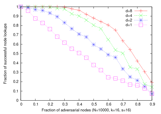
One has to wonder about their sample sizes, but the shapes of the curves are still (more or less) evident. For \(d = 8\) disjoint lookup paths, it can be seen that the probability of success is still around 0.9 when Sybil peers account for half of the network, and stays strong until the fraction of adversarial nodes reaches about 0.75.

Combining Results

Successfully retrieving data from a DHT depends on a successful lookup and on the lookup set containing at least one honest peer. If we treat these two events as independent, we can model our overall probability of success as \(P \cdot \operatorname{E}[R_{L,k}]\).

The shape of this combined distribution depends on the distribution of lookup path lengths, which is why I haven’t plotted it here. Further research is needed to determine whether breaking the one-to-one correspondence between peers and nodes significantly impacts the established models for path length distribution, and if so, how.

The good news is that we now have a complete model for how certain DHTs fare under Sybil attacks. We also have a list of parameters we can tune to increase the network’s resilience in the face of attacks, and we can quantify exactly how much of a difference any given change will make.

One last defensive measure: Say you want to store data at some address \(A\), but the network is currently under a heavy Sybil attack, and you estimate \(P \cdot \operatorname{E}[R_{L,k}] \approx 0.4\), meaning you have a 40% chance of successfully storing data at \(A\) and other peers have a 40% chance of successfully retrieving it. This is likely not good enough. OK then - just use some other addresses. For instance you could derive \(A_1 = \operatorname{H}(A \vert 1), A_2 = \operatorname{H}(A \vert 2)\), etc.²⁶ If the probability of either of those addresses failing is \(1-0.4 = 0.6\), then the probability of both failing is \(0.6^2 = 0.36\). If you use five addresses, then your chances of success are back over 90% - even while the DHT is more than halfway compromised!

Of course, countermeasures like this rely on the assumption that the DHT is usually operating well under its carrying capacity, since going from one address to five addresses really just amounts to increasing data redundancy fivefold. In a sense, increasing \(k\) is also a way of increasing data redundancy, since data for any address is stored on the \(k\) closest peers to that address - though increasing \(k\) impacts other parts of the system as well (most notably routing). In any case, as noted above, most modern systems are operating far under their capacity limit, so there is room for experimentation here, and optimizing the allocation of these spare resources may be an interesting avenue for future research..

Closing Thoughts

Ad-hoc, peer-to-peer distributed systems had a moment in the early 2000s. This was the era that brought us Freenet, BitTorrent, I2P, and many other systems like them. Most of these have fallen out of fashion in favor of centralized technologies, in part because centralized systems swap out Sybil vulnerability for several less-obvious issues (I’ve written about this trend and its implications here). This shift in fashion has led most people to discount these peer-to-peer systems – aside from BitTorrent – as novelties at best.

I think that is a big mistake. It’s easy to forget that the tech landscape was very different in the early 2000s. Spare memory and CPU cycles were hard to come by. The good news is, those days are over. It’s only relatively recently that we’ve reached a point where almost all machines²⁷ running DHT peers can be expected to have spare RAM on the order of gigabytes. Thus these redundancy-focused Sybil countermeasures are viable today to a degree that they never have been before.

We can design ad-hoc peer-to-peer systems which detect and resist malicious activity without interrupting normal operation. We can make these systems performant, and we can make them reliable to within arbitrary tolerances. We can make these systems today. So what are we waiting for?

---